🔬 Lab 1: Least Squares

Before starting this lab, please review the following tutorials: Python Basic, Python Intermediate, and Numpy.

• Python Basic: While you may already be familiar with much of this material, it’s recommended to review it as a refresher.

• Python Intermediate: Go through this tutorial carefully. Many past ECE487 cadets lacked familiarity with the topics covered here.

• NumPy: We will be using NumPy extensively in this class. A solid understanding of this tutorial is highly recommended.

Least Sqaures Estimation

In this lab, we will solve a least squares regression problem to find the best-fit linear equation for a set of measured data. Let the measured data be represented by \(\mathbf{t} = (t_1, t_2, \cdots, t_n)\), with corresponding input values \(\mathbf{x} = (x_1, x_2, \cdots, x_n)\).

Our goal is to find \(w_1\) and \(w_0\) such that the equation \(t = w_1x + w_0\) best approximates the linear relationship between \(x\) and \(t\).

Plotting the Data

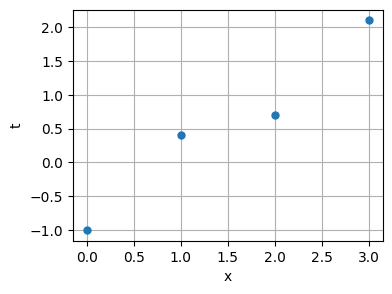
First, let’s visualize the data:

import numpy as np
import matplotlib.pyplot as plt

x = np.array([0, 1, 2, 3])
t = np.array([-1, 0.4, 0.7, 2.1])

fig = plt.figure(figsize=(4, 3))
ax = fig.add_subplot()

plt.plot(x, t, "o", markersize=5)
plt.xlabel("x")
plt.ylabel("t")
plt.grid(True)
plt.show()

Linear Equation in Matrix Form

We can express the linear equation in matrix form as \(t = \mathbf{c} \cdot \mathbf{w}\), where:

\(\mathbf{c} = \begin{bmatrix} x & 1 \end{bmatrix}\) and \(\mathbf{w} = \begin{bmatrix} w_1 \ w_0 \end{bmatrix}\). This gives us:

\(t = w_1x + w_0 = \begin{bmatrix} x & 1 \end{bmatrix} \begin{bmatrix} w_1 \ w_0 \end{bmatrix} = \mathbf{c} \cdot \mathbf{w}\).

Given \(\mathbf{x} = (x_1, x_2, \cdots, x_n)\) and \(\mathbf{t} = (t_1, t_2, \cdots, t_n)\), we can set up the following system of equations:

\(\begin{bmatrix} -1 \ 0.4 \ 0.7 \ 2.1 \end{bmatrix} = \begin{bmatrix} 0 & 1 \ 1 & 1 \ 2 & 1 \ 3 & 1 \end{bmatrix} \begin{bmatrix} w_1 \ w_0 \end{bmatrix}\),

or, in matrix notation, \(\mathbf{t} = \mathbf{C}\mathbf{w}\).

Here:

\(\mathbf{C} = \begin{bmatrix} x_1 & 1 \ x_2 & 1 \ x_3 & 1 \ x_4 & 1 \end{bmatrix} = \begin{bmatrix} 0 & 1 \ 1 & 1 \ 2 & 1 \ 3 & 1 \end{bmatrix}\).

Creating the Matrix \(\mathbf{C}\)

We can create the \(C\) matrix using np.column_stack

ones = np.ones_like(x)  # Create an array of ones with the same shape as x
C = np.column_stack((x, ones))  # Combine x and ones as columns
print(C)

[[0 1]
 [1 1]
 [2 1]
 [3 1]]

Solving for \(\mathbf{w}\) Using np.linalg.lstsq

Next, we can use the np.linalg.lstsq function to solve for \(\mathbf{w}\):

w = np.linalg.lstsq(C, t, rcond=None)[0]
print(w)
# Or you can extract the individual coefficients
w1, w0 = np.linalg.lstsq(C, t, rcond=None)[0]
print(w1, w0)

[ 0.96 -0.89]
0.9599999999999999 -0.8899999999999998

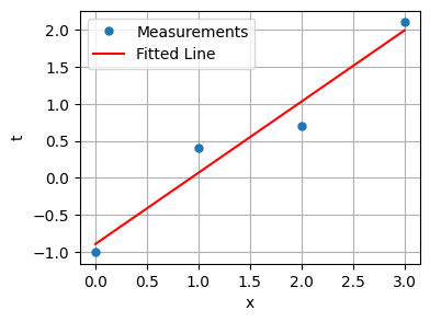
With \(w_1 = 0.96\) and \(w_0 = -0.89\), the best-fitting line is:

\(t = 0.96x - 0.89\)

Plotting the Fitted Line

Now, let’s plot the fitted line alongside the data points:

fig = plt.figure(figsize=(4, 3))
ax = fig.add_subplot()

plt.plot(x, t, "o", label="Measurements", markersize=5)
plt.plot(x, w1 * x + w0, "r", label="Fitted Line")
plt.xlabel("x")
plt.ylabel("t")
plt.legend()
plt.grid(True)
plt.show()

💻 Procedure

Update Your Code

1. Navigate to the ECE487 workspace, ece487_wksp.

2. Right-click on the ece487_wksp folder and choose Git Bash Here from the menu.

3. To pull the latest updates, run the following command:

git pull upstream main

Galilei’s Falling Body Experiment

1. Open the falling_body.ipynb notebook in VS Code.

2. Carefully review the contents of this notebook to understand the three different techniques used for curve fitting.

Deliverables

1. Open the Lab1_LSE.ipynb notebook using VS Code.

2. Follow the instructions within the notebook to complete your code.

3. Push your code to your GitHub repository and submit the output plot in Gradescope.