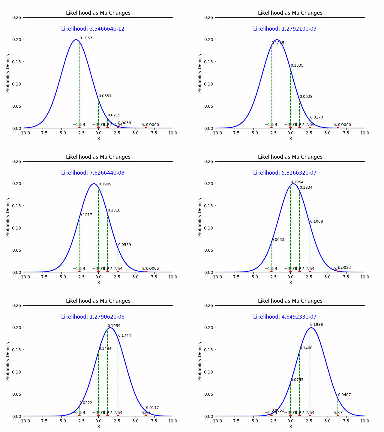
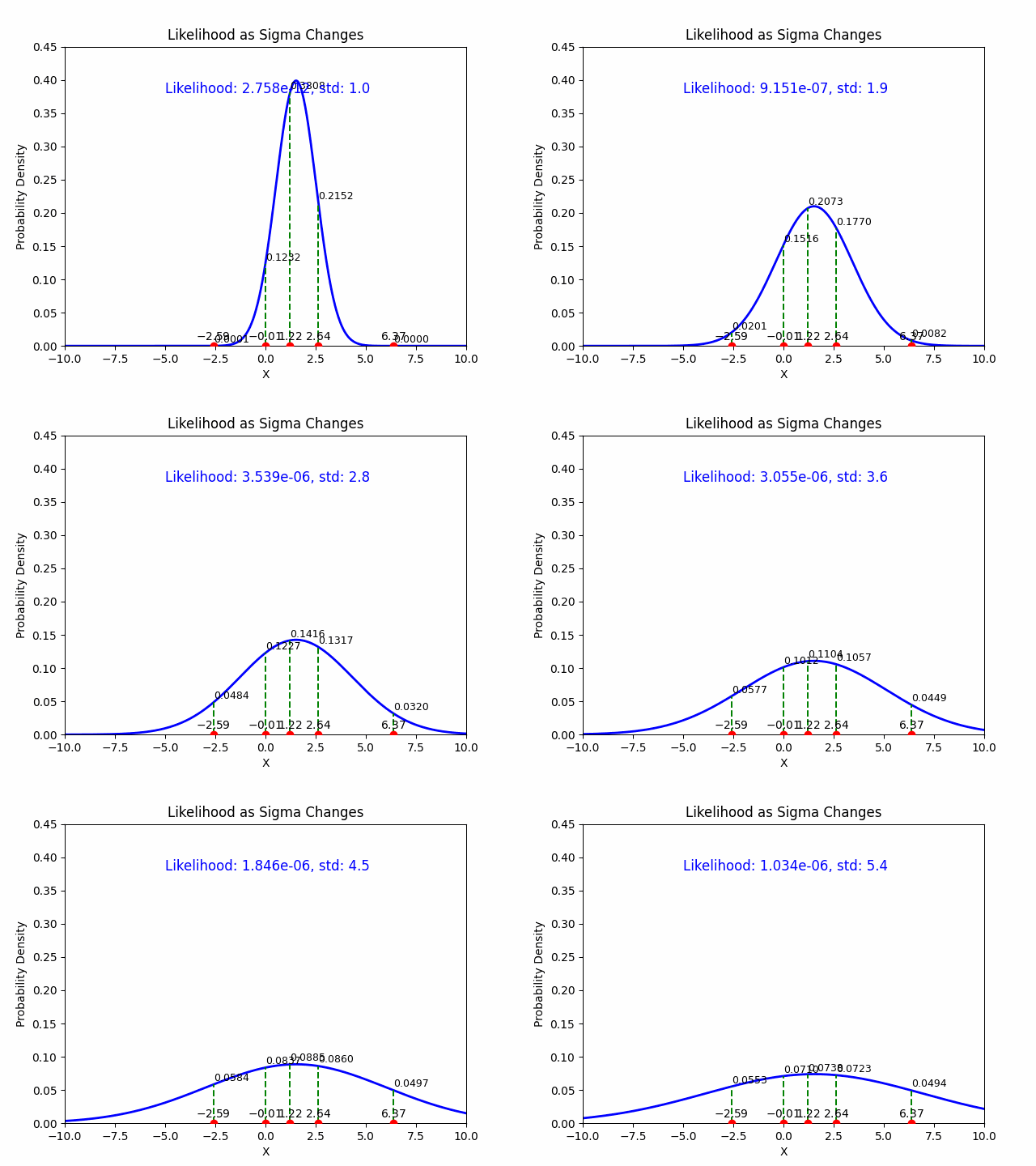
Maximum Likelihood Estimation (MLE)

Maximum Likelihood Estimation (MLE)#

Likelihood function#

The likelihood function is a fundamental concept in statistical inference and is defined as a function that measures how well a set of parameters explains a given set of data. Specifically, for a set of observed data and a statistical model with certain parameters, the likelihood function gives the probability (or probability density) of observing the data, viewed as a function of the parameters.

Definition#

For a set of observed data $\mathcal{D} = (y_1, y_2, ..., y_n)$ and a statistical model with a probability distribution $f(y \mid \theta)$ parameterized by $\theta$, the likelihood function $L(\theta \mid \mathcal{D})$ is:

\[L(\theta \mid \mathcal{D}) = f(\mathcal{D} \mid \theta)\]

Here:

$\mathcal{D}$ represents the observed data.
$\theta$ represents the parameters of the model.
$f(\mathcal{D} \mid \theta)$ is the probability (for discrete data) or the probability density (for continuous data) of the observed data given the parameters.

For independent and identically distributed (i.i.d.) data, where each $y_i$ is drawn from the same distribution $f(y \mid \theta)$, the likelihood function is often written as the product of the individual probabilities (or densities):

\[L(\theta \mid \mathcal{D}) = \prod_{i=1}^{n} f(y_i \mid \theta)\]

Example:#

If you have a set of observed coin flips, and you are trying to estimate the probability $p$ of landing heads, the likelihood function would measure how likely the observed flips (e.g., 7 heads and 3 tails) are, given different values of $p$. You’d adjust $p$ to maximize this likelihood, which leads to the method of maximum likelihood estimation (MLE).

In summary, the likelihood function is the probability of the observed data treated as a function of the model’s parameters, and it forms the foundation for parameter estimation in many statistical methods, including MLE.

Likelihood vs. probability#

Likelihood and probability are related concepts but serve different purposes in statistics and have distinct interpretations:

1. Probability:#

Definition: Probability measures the chance that a certain event or outcome will occur, given a fixed model and parameters.
Interpretation: It answers the question: Given the model and parameters, what is the probability of observing this specific outcome?
Example: Suppose you flip a biased coin with a known probability of heads $p = 0.7$. The probability of getting heads in a single flip is 0.7.

In formula terms:

\[P(X = x \mid \theta) \quad \text{(The probability of observing outcome } x \text{ given parameter } \theta)\]

where $X$ is a random variable representing an outcome, and $\theta$ is the fixed parameter (e.g., the bias of the coin).

2. Likelihood:#

Definition: Likelihood measures how well a particular set of parameters explains the observed data. It is viewed as a function of the parameters, given the data.
Interpretation: It answers the question: Given this observed data, how likely is it that a particular set of parameters generated it?
Example: Imagine you observe 7 heads out of 10 flips and want to estimate the probability $p$ of heads for this biased coin. The likelihood function will give you the “likelihood” of different values of $p$, given that you’ve observed 7 heads in 10 flips. You would adjust $p$ to find the value that maximizes this likelihood, using Maximum Likelihood Estimation (MLE).

In formula terms:

\[L(\theta \mid \mathcal{D}) = P(\mathcal{D} \mid \theta) \quad \text{(The likelihood of parameter } \theta \text{ given the data } \mathcal{D})\]

where $\mathcal{D} =(y_1, y_2, ..., y_n)$ is the observed data, and $\theta$ is the variable parameter to be estimated.

3. Key Differences:#

Perspective:
- Probability is used when the parameters $\theta$ are fixed, and we want to find the probability of observing certain data or outcomes.
- Likelihood is used when the data $\mathcal{D}$ are fixed, and we are varying the parameters $\theta$ to find the values that make the data most probable.
What Changes:
- In probability, the parameters are fixed, and you consider the probability of different outcomes.
- In likelihood, the data is fixed, and you consider different possible parameter values to see which one makes the data most probable.
Use Cases:
- Probability is typically used in forward problems where you’re predicting outcomes based on a model (e.g., predicting the probability of heads in a coin flip).
- Likelihood is used in parameter estimation (e.g., finding the value of $p$ in a coin-flip experiment that best explains the observed data).
Summary
- Probability is forward-looking: If you know the parameters of a situation, you can calculate the probability of various outcomes. It’s like saying, “Given that the die is fair, what is the chance I’ll roll a six?”
- Likelihood is reverse-engineering: Given an outcome, likelihood tells us how plausible different parameter values are. It’s like saying, “Given that I rolled a six, how plausible is it that my die is fair?”
- So, when you toss a coin, the probability tells you the chance of heads or tails. But if you get ten heads in a row, likelihood helps you figure out if the coin is fair or biased.

4. Example:#

Probability: Given a coin with $p = 0.7$ (where $p$ is the fixed probability of heads), the probability of flipping 7 heads out of 10 flips is computed based on this known $p$.
Likelihood: If you observe 7 heads out of 10 flips and don’t know $p$, the likelihood function tells you how likely different values of $p$ are, given this outcome. You might use MLE to estimate the most likely value of $p$.

In short, probability is about predicting outcomes from known parameters, while likelihood is about estimating parameters from observed outcomes.

5. Likelihood in MLE#

In the context of Maximum Likelihood Estimation (MLE), likelihood is a function that measures how well a particular set of parameters explains the observed data. Given observed data points, the likelihood function evaluates the plausibility of different parameter values of a statistical model. MLE aims to find the parameter values that maximize this likelihood function, effectively making the observed data most probable under those parameters.

So, imagine you have data on how often students pass an exam based on study hours. The likelihood function helps you figure out the parameters (like the average study hours) that make your observed data (exam pass rates) most likely.

MLE Example#

To estimate the mean and standard deviation of a set of data $\mathcal{D} = \{y_1, y_2, \dots, y_N\}$, assuming that the $y$’s are drawn from a Gaussian (normal) distribution, we can use Maximum Likelihood Estimation (MLE).

1. Problem Setup:#

Assume that the data $\mathcal{D} = \{y_1, y_2, \dots, y_N\}$ comes from a Gaussian distribution with unknown mean $\mu$ and unknown standard deviation $\sigma$. The probability density function (PDF) for a normal distribution is:

\[f(y_i \mid \mu, \sigma) = \frac{1}{\sqrt{2\pi\sigma^2}} \exp\left( -\frac{(y_i - \mu)^2}{2\sigma^2} \right)\]

2. Likelihood Function:#

The likelihood function $L(\mu, \sigma \mid \mathcal{D})$ for the Gaussian distribution, given the data $\mathcal{D}$, is the product of the probabilities (or densities) of each individual observation $y_i$ under the Gaussian model:

\[L(\mu, \sigma \mid \mathcal{D}) = \prod_{i=1}^{N} f(y_i \mid \mu, \sigma)\]

Substituting the PDF of the Gaussian distribution:

\[L(\mu, \sigma \mid \mathcal{D}) = \prod_{i=1}^{N} \frac{1}{\sqrt{2\pi\sigma^2}} \exp\left( -\frac{(y_i - \mu)^2}{2\sigma^2} \right)\]

3. Log-Likelihood Function:#

It is common to maximize the log-likelihood instead of the likelihood, as it simplifies the math (turning products into sums). The log-likelihood function $LL(\mu, \sigma \mid \mathcal{D})$ is:

\[LL(\mu, \sigma \mid \mathcal{D}) = \log L(\mu, \sigma \mid \mathcal{D})\]

Taking the logarithm:

\[LL(\mu, \sigma \mid \mathcal{D}) = \sum_{i=1}^{N} \log \left( \frac{1}{\sqrt{2\pi\sigma^2}} \exp\left( -\frac{(y_i - \mu)^2}{2\sigma^2} \right) \right)\]

This simplifies to:

\[LL(\mu, \sigma \mid \mathcal{D}) = -\frac{N}{2} \log(2\pi) - N \log(\sigma) - \frac{1}{2\sigma^2} \sum_{i=1}^{N} (y_i - \mu)^2\]

4. Maximizing the Log-Likelihood:#

Now, we find the values of $\mu$ and $\sigma$ that maximize the log-likelihood by taking the partial derivatives with respect to $\mu$ and $\sigma$, and setting them to zero.

(a) Derivative with respect to $\mu$:#

\[ \frac{\partial}{\partial \mu} LL(\mu, \sigma \mid D) = \frac{1}{\sigma^2} \sum_{i=1}^{N} (y_i - \mu)\]

Setting this equal to zero:

\[\sum_{i=1}^{N} (y_i - \mu) = 0\]

Solving for $\mu$:

\[\hat{\mu} = \frac{1}{N} \sum_{i=1}^{N} y_i\]

Thus, the MLE estimate for $\mu$ is the sample mean.

(b) Derivative with respect to $\sigma$:#

\[ \frac{\partial}{\partial \sigma} LL(\mu, \sigma \mid D) = -\frac{N}{\sigma} + \frac{1}{\sigma^3} \sum_{i=1}^{N} (y_i - \mu)^2\]

Setting this equal to zero:

\[-\frac{N}{\sigma} + \frac{1}{\sigma^3} \sum_{i=1}^{N} (y_i - \mu)^2 = 0\]

Multiplying by $\sigma^3$ and solving for $\sigma^2$:

\[\sigma^2 = \frac{1}{N} \sum_{i=1}^{N} (y_i - \mu)^2\]

Thus, the MLE estimate for $\sigma^2$ is the sample variance. Taking the square root gives the MLE estimate for $\sigma$:

\[\hat{\sigma} = \sqrt{\frac{1}{N} \sum_{i=1}^{N} (y_i - \hat{\mu})^2}\]

5. Summary of MLE Estimates:#

The MLE estimate for the mean $\mu$ is: $$\hat{\mu} = \frac{1}{N} \sum_{i=1}^{N} y_i \quad \text{(the sample mean)}$$
The MLE estimate for the standard deviation $\sigma$ is: $$\hat{\sigma} = \sqrt{\frac{1}{N} \sum_{i=1}^{N} (y_i - \hat{\mu})^2} \quad \text{(the sample standard deviation)}$$

These are the maximum likelihood estimates of the mean and standard deviation for data drawn from a Gaussian distribution.