🔬 Lab10: CV

🔬 Lab10: CV#

📌 Objectives#

Students should be able to explain how Histogram of Oriented Gradients (HOG) features enable object detection.
Students should be able to train and test a custom stop sign detector using Dlib and evaluate its accuracy.
Students should be able to stream and process live camera images in ROS 2 using usb_cam and OpenCV.
Students should be able to implement a ROS node to detect stop signs in real time and estimate their distance.

📜 Overview#

In this lab, we explore how the Histogram of Oriented Gradients (HOG) features, combined with a Support Vector Machine (SVM), enable object detection. By now, we’re all familiar with histograms, but in this context, they help simplify an image so a computer can quickly and accurately identify objects within it.

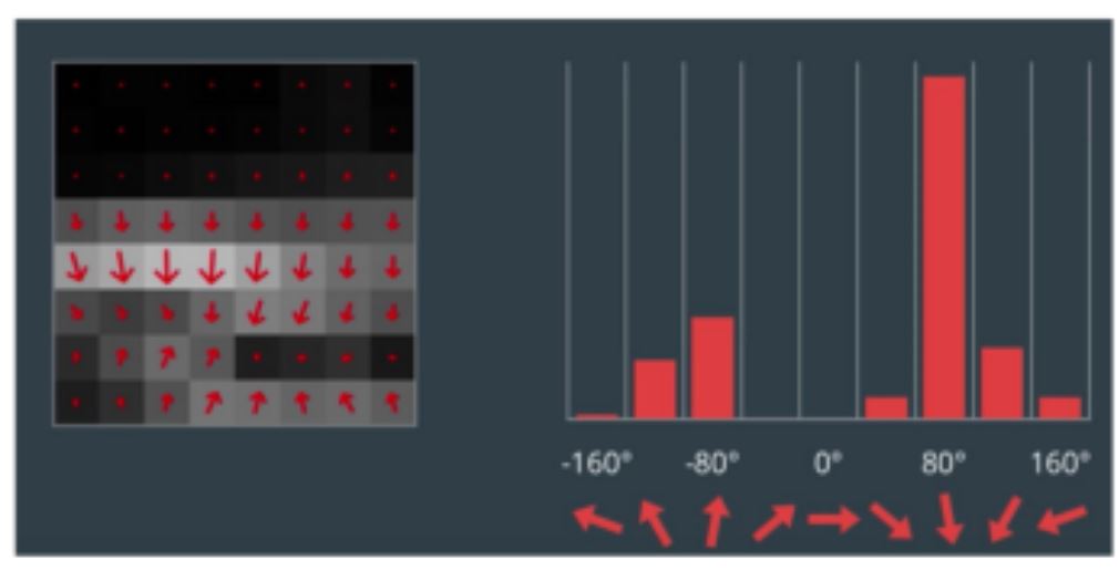
Rather than analyzing the gradient direction of every single pixel, HOG groups pixels into small cells. Within each cell, the gradient directions are computed and categorized into orientation bins, with stronger gradients carrying more weight. This approach helps reduce the influence of random noise and provides a structured representation of the image. HOG features maintain the distinct shape of an object while allowing for slight variations. For instance, consider an object detector designed to recognize a car:

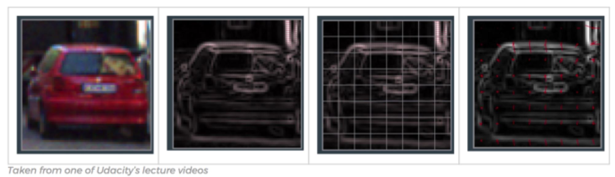
Comparing each individual pixel of this training image with another test image would not only be time consuming, but it would also be highly subject to noise. As previously mentioned, the HOG feature will consider a block of pixels. The size of this block is variable and will naturally impact both accuracy and speed of execution for the algorithm. Once the block size is determined, the gradient for each pixel within the block is computed. Once the gradients are computed for a block, the entire cell can then be represented by this histogram. Not only does this reduce the amount of data to compare with a test image, but it also reduces the impacts of noise in the image and measurements.

Now that we understand HOG features, let’s leverage OpenCV and Dlib to build a stop sign detector. First, we need to download a repository containing pre-made test and training data. Keep in mind that we won’t evaluate the algorithm’s effectiveness using the training data—it’s expected to perform well there. Instead, our goal is to use a diverse test set to develop a detector robust enough to recognize stop signs in new images.

🌱 Pre-Lab: ROS2 Client Libraries#

Create a package named lab10_cv with the BSD-3-Clause license and dependencies:
- rclpy
- cv_bridge
- sensor_msgs
- std_msgs
- opencv2
Hint: There’s a way to include all dependencies at the time of package creation.
Download the lab10_prelab.tar.xz. Extract the files and move them to ~/master_ws/src/ece387_ws/lab10_cv/test.
Open the Jupyter Notebook file, lab10_prelab.ipynb with vscode.
Click Select Kernel in the top right corner, choose Python Environments, and select /usr/bin/python3.
As you read through the notebook, run the python code by clicking the arrow button in the top left corner.
If the following message pops up, choose Install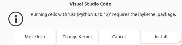
Take a screenshot of the gradient image and submit it on Gradescope.

🧪 Lab Instructions: Object Detection Using HOG and ROS#

In this lab, you’ll build a stop sign detector using HOG (Histogram of Oriented Gradients) features, test it, and integrate it with a ROS-based camera system.

1. Build a Detector Using HOG Features#

Open a terminal and download the demo repository:

cd ~/master_ws/src
git clone git@github.com:ECE495/HOG_Demo.git
cd HOG_Demo

Inside the repo, you’ll find folders for training and test images. We’ll use a tool called imglab to annotate the training images.
Go to imglab in your browser.
When prompted, click “UMM, MAYBE NEXT TIME!” to skip the sign-in.
In the bottom left corner, click load, select the training folder from your local files, and then click upload. This should load 19 images.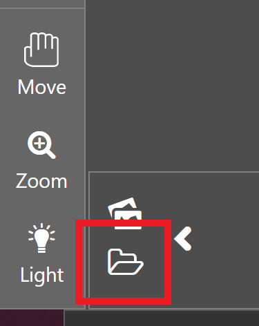
Select the Rectangle tool and begin labeling stop signs:
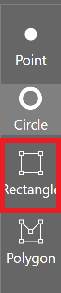
- Click and drag to draw a bounding box only around each stop sign.
- If an image contains multiple stop signs, draw a box around each.
- If you make a mistake, select the box and press delete.
Note

It is important to label all examples of objects in an image; otherwise, Dlib will implicitly assume that regions not labeled are regions that should not be detected (i.e., hard-negative mining applied during extraction time).

Tip

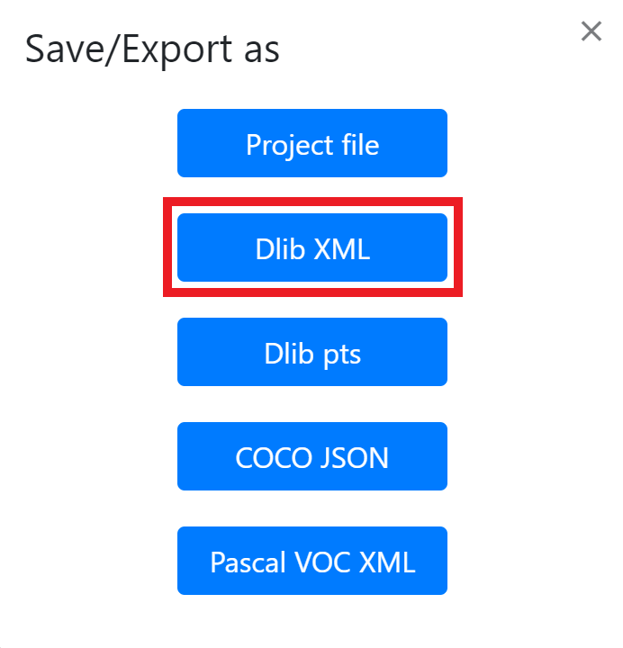
Use Alt + ←/→ to switch between images.
Once you’ve labeled all images, press Ctrl + e to export your annotations.
- Save the file as stop_annotations.xml in the training folder.

Create a Python script:

cd ~/master_ws/src/HOG_Demo
touch trainDetector.py

Open it in your preferred code editor and paste in the following code:

# Import required libraries
import argparse  # For parsing command-line arguments
import dlib      # For training and testing the object detector

# Set up command-line arguments
ap = argparse.ArgumentParser()
ap.add_argument("-x", "--xml", required=True, help="Path to input XML file")          # Path to the labeled training dataset in XML format
ap.add_argument("-d", "--detector", required=True, help="Path to output detector (.svm)")  # Path where the trained .svm model will be saved
args = vars(ap.parse_args())  # Parse the arguments into a dictionary

# Inform the user that training is starting
print("[INFO] Training detector...")

# Set training options for the object detector
options = dlib.simple_object_detector_training_options()
options.C = 1.0               # Regularization parameter; higher values = lower bias, higher variance
options.num_threads = 4      # Number of CPU threads to use for training
options.be_verbose = True    # Print progress and training status to the console

# Train the detector using the specified XML file and save the model
dlib.train_simple_object_detector(args["xml"], args["detector"], options)

# After training, test the detector on the training dataset to evaluate performance
print("[INFO] Training accuracy: {}".format(
    dlib.test_simple_object_detector(args["xml"], args["detector"])))

# Load the trained detector from disk
detector = dlib.simple_object_detector(args["detector"])

# Create a window to visualize the learned detector's HOG features
win = dlib.image_window()
win.set_image(detector)  # Show the detector as a HOG filter visualization

# Wait for the user to hit Enter before closing
dlib.hit_enter_to_continue()

Run the script to train your detector:
```
python3 trainDetector.py --xml training/stop_annotations.xml --detector training/stop_detector.svm
```
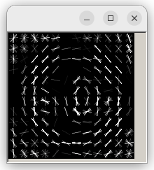
You may get a few errors pop up during execution based on your choice for bounding boxes. Make sure you address those errors before continuing. If everything runs correctly, you’ll see a visualization of the trained HOG filter as shown below. If you get an error, double-check your annotations and fix any issues.

2. Test the Detector#

Now it is time to build our code to test the detector.

Create a new Python script:

cd ~/master_ws/src/HOG_Demo
touch testDetector.py

Add the following code:

# Import the necessary packages
from imutils import paths   # Utility to easily grab file paths from a directory
import argparse             # Used to handle command-line arguments
import dlib                 # Library for machine learning tools including object detection
import cv2                  # OpenCV for image processing

# Set up command-line arguments
ap = argparse.ArgumentParser()
ap.add_argument("-d", "--detector", required=True, help="Path to trained detector (.svm)")
ap.add_argument("-t", "--testing", required=True, help="Path to testing images folder")
args = vars(ap.parse_args())  # Parse the arguments into a dictionary

# Load the trained detector using the path provided
# The .svm file contains the learned HOG + SVM model
detector = dlib.simple_object_detector(args["detector"])

# Loop through each image file in the testing directory
for imagePath in paths.list_images(args["testing"]):

    # Read the image from disk using OpenCV
    image = cv2.imread(imagePath)

    # Convert the image from BGR (OpenCV default) to RGB (required by dlib)
    # Then, pass it to the detector which returns a list of bounding boxes
    boxes = detector(cv2.cvtColor(image, cv2.COLOR_BGR2RGB))

    # Loop through each bounding box returned by the detector
    for b in boxes:
        # Get the coordinates of the bounding box
        (x, y, w, h) = (b.left(), b.top(), b.right(), b.bottom())

        # Draw the bounding box on the image using a green rectangle
        # (x, y) is the top-left, (w, h) is the bottom-right corner
        cv2.rectangle(image, (x, y), (w, h), (0, 255, 0), 2)

    # Display the image with the detections in a pop-up window
    cv2.imshow("Detection", image)

    # Wait for a key press before moving to the next image
    # (0 means wait indefinitely until a key is pressed)
    cv2.waitKey(0)

Run your test:

python3 testDetector.py --detector training/stop_detector.svm --testing test

Look at your results. Did the detector work well? Were there any false positives or missed signs?

3. ROS: Live Camera Streaming#

ROS includes several tools for working with commercial off-the-shelf cameras, like the USB camera on your robot. The main one we’ll use is the usb_cam package, which is already installed. We’ll now use ROS 2 and usb_cam to stream live video from the camera.

SSH into your robot and run:

ros2 run usb_cam usb_cam_node_exe --ros-args -p video_device:=/dev/video0

If you have an error that can’t find the usb_cam package, install the package using

sudo apt install ros-humble-usb-cam

If you have a permission error, you need to run

sudo usermod -aG video $USER
sudo reboot now

Ignore any calibration error messages — we’ll handle that later.

On your Master PC, Run:
```
ros2 topic list
```
You should see topics like /image_raw, /camera_info, etc.

Check topic bandwidth:

ros2 topic bw /image_raw
ros2 topic bw /image_raw/compressed

Check image publishing rate:

ros2 topic hz /image_raw
ros2 topic bw /image_raw/compressed

View the camera feed:
```
ros2 run rqt_image_view rqt_image_view
```
Select /image_raw to see the feed. Try waving your hand in front of the camera to check latency.
You may have noticed that streaming images over WiFi is quite slow. While using compressed images can help, it also increases the processing load on both the Raspberry Pi and the master computer. To avoid this during development, we’ll run camera-related code directly on the master computer. Once everything is working, we can move the code back to the robot.
Disconnect the camera from the robot and plug it into the master computer. You can also unplug the gamepad—it’s not needed for now.

On the master computer, run the following command to start the camera node:

ros2 run usb_cam usb_cam_node_exe --ros-args -p video_device:=/dev/video0

Check topic bandwidth and image publishing rate:

ros2 topic bw /image_raw
ros2 topic hz /image_raw

To verify the image stream, launch the image viewer:
```
ros2 run rqt_image_view rqt_image_view
```

4. Capture Training Images with ROS#

You’ll now use a script to save training images of stop signs from your live feed.

Download the image_capture.py script and place it in your package’s script folder.
Update your setup.py to include the script as an entry point. This is necessary to ensure that the script runs as a node.
Open the image_capture.py script and read through the code carefully. It may be unfamiliar, but take your time to understand what each part is doing.
Rebuild your package:
```
ccbuild --packages-selelct labl0-cv
```

Run the USB camera node on Master:

ros2 run usb_cam usb_cam_node_exe --ros-args -p video_device:=/dev/video0

Open a new terminal, navigate to the Documents directory, and run
```
ros2 run lab10_cv image_capture -o ./training_images/
```
Press s and Enter to save an image. Take multiple images from different angles and distances. Press Ctrl + C when done.
Use imglab again to annotate your new images and save the XML file as before. Then re-train your detector using the updated dataset.

5. Use the Detector in a ROS Node#

In this step, you’ll create a ROS 2 node that runs your stop sign detector in real-time using the live camera feed.

Download the stop_detector.py script and place it in your package’s script folder.
Update your setup.py to include the script as an entry point.
Edit stop_detector.py.
- Inside the camera_callback() function, use the same image processing approach used in the image_capture.py script to convert ROS image messages into OpenCV format (cv_image).
- Apply your HOG-based detector to the cv_image, just like you did in Test the Detector.
- Draw bounding boxes around any detected stop signs. Use the cv2.rectangle function to draw the boxes.
- Use cv2.imshow() to display the video, and make sure to call cv2.waitKey(1) to allow the video to refresh in real-time.
Use the following command, replacing <path/to/detector> with the path to your trained .svm detector file:
```
ros2 run lab10_cv stop_detector -d <path/to/detector>
```
You should now see a window displaying the camera feed with stop signs outlined.

Install OBS Studio to record your stop sign detection in action.

sudo apt update
sudo apt install obs-studio qtwayland5

Run obs from the terminal, or find it under Applications.
Set up recording:
- In the Scenes panel (bottom-left), click the + and name your scene (e.g., “Stop Sign Detection”).
- In the Sources panel, click the + and choose Window Capture.
- Select the window showing your detector output.
- Click Start Recording.
Move around while keeping the stop sign visible to showcase detection capabilities. Present the stop sign from different angles, including varied pan, tilt, and rotation positions, as demonstrated in the video below.
When finished, click Stop Recording.
Upload your recording to the class Teams channel.

6. Estimating Distance to a Stop Sign#

In this section, you’ll determine the distance between the stop sign and the camera using its known size and a detector.

Calculate the Camera’s Focal Length: Start with a stop sign that has a known width, \(Y\), positioned at a known distance, \(Z\), from the camera. The detector identifies the stop sign and provides its perceived width in pixels, \(y\). Using these values, calculate the camera’s focal length, \(f\), with the following formula:

\[f = Z \times \frac{y}{Y}\]

To determine the focal length, print the perceived width of the stop sign, \(y\).
Estimate the Distance to the Stop Sign: Once you have the calculated focal length, \(f\), use it along with the known width of the stop sign, \(Y\), and its perceived width in pixels, \(y\), to compute the distance from the camera using this formula:

\[Z = f \times \frac{Y}{y}\]
Implement a Class for Distance Calculation
- Define two class variables:
  - FOCAL: The calculated focal length.
  - STOP_WIDTH: The known width of the stop sign.
- Create a class function named get_distance, which calculates the distance using the FOCAL length and STOP_WIDTH.
Tip

Pay attention to the x and w variables in the box—understanding their role is crucial!
Publish the Distance
- Set up a publisher to send the calculated distance using Float32 messages from the std_msgs package on the /stop_dist topic.
- Ensure the published distance reflects every detected object in the image.

🚚 Deliverables#

[15 Points] Complete the stop_detector.py Script
- Ensure the script is fully functional and implements all required features.
- Push your code to GitHub and confirm that it has been successfully uploaded. NOTE: If the instructor can’t find your code in your repository, you will receive a grade of 0 for the coding part.
[10 Points] Submit Screenshots
- Submit the screenshot of the gradient image from the pre-lab Jupyter notebook.
[15 Points] Demonstration
- Show the stop_detector node successfully detect the stop sign.
- OBS recording showing real-time stop sign detection (upload to Teams).
- Must include varied angles/distances and display bounding boxes.
- Published distances on /stop_dist (verified via ros2 topic echo).
[10 points] Summary
- Brief summary of HOG principles, challenges faced, and detection accuracy.